Fighting JPEG color banding

If you ever tried to save photos to JPEG format, you probably know how bad JPEGs can look. Decades of domination of this format have led to most internet users having an allergy to effects called “JPEG artifacts.”

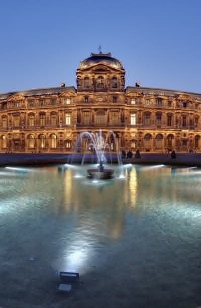
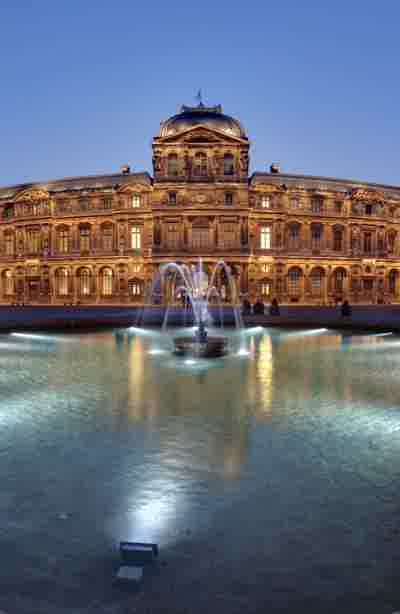
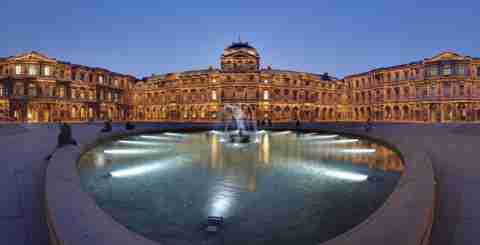Louvre. 480×245px, heavily compressed JPEG

No doubt, no one wants to share such a mess with someone else. If you ask me what exactly is wrong with the image, I’d probably say that in general it looks very close to the original: no significant color shift, all objects are distinguishable. However, I’d say there are two major problems:

1. Soft gradients look like separate blocks or bands. That is why it is called color banding. This is especially noticeable on the sky, but you can see the same on the ground.

2. There are parasite color gradients around sharp objects (look at the roof), and other tiny elements. This effect is called ringing.

Let me show you some magic. I’d like to apply these effects separately.

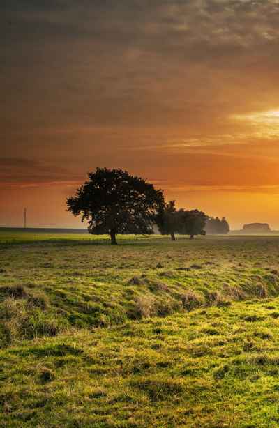
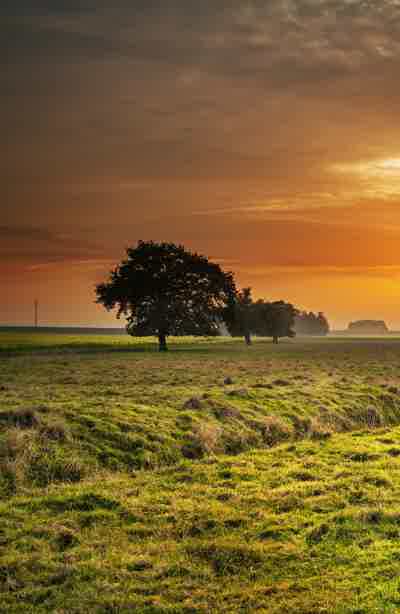
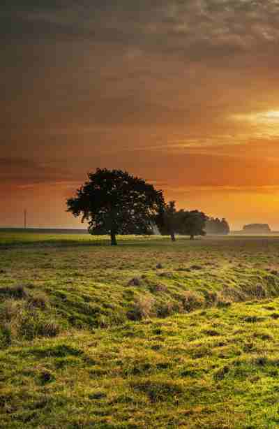
So, the left image is a reference with perfect quality. The center image is heavily compressed, but only has ringing artifacts, while the image on the right has only color banding. All three images are actual JPEGs, crafted with the unmodified libjpeg library, no Photoshop involved.

Both ringing, and banding images are still looking unacceptable. However, there is a trick, I actually slightly scaled the samples on the page. You are looking at 480 pixels wide image in total, while it occupies 600 CSS pixels (if you’re reading this on a desktop). So the pixel density is 0.8x. Modern screens often have pixel density 2x and more. A common technique is delivering an image with a 2x density (compared to CSS pixels), with minimum possible quality.

So what’ll be changed if we try to do the same for 2x pixels density? The samples are the same but with higher resolution: original, heavily compressed with ringing only artifacts, and banding only.

I’m wondering, have you thought there is a mistake for a second? There is no mistake, the center sample indeed looks perfect, like the original. In contrast, the right sample looks as ugly as it was on 0.8x density.

It’s amazing that the human eye is not sensitive to ringing on a small scales. If you zoom in the page you’ll see that heavy ringing is still here. We just don’t see the effect.

The problem

The fact that we don’t see ringing is quite interesting, what value can we get here? The key is above. For 2x density we need to choose “minimum possible quality” (this is also true for any density). We have to choose a quality which will not introduce significant artifacts.

The problem is when reducing quality, both ringing and color banding appears on the image. In practice, for 2x density it means that we often have to choose a quality which will not introduce significant color banding.

What if we could reduce quality, and bitrate even more without introducing significant color banding?

To answer this question, we need to dive into how JPEG compression works first. Don’t worry, this topic will be extremely simplified.

JPEG compression quick tour

First you need to know, JPEG compresses an image by small blocks, 8×8 pixels. You can even notice blocks on any heavily compressed sample on this page. Also yes, banding boundaries are always 8 pixels size.

The JPEG codec doesn’t store pixels’ values directly. Instead, each block is compared to 64 possible frequency patterns, and only coefficients per pattern per color channel is stored in the file. You can read the JPEG Quality Loss article if you need further explanation.

So, look at the table:

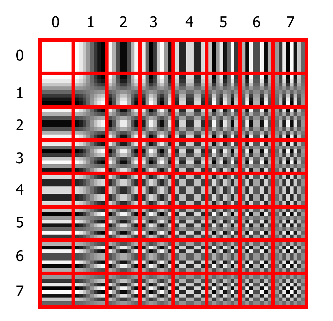The frequency patterns for 8×8 block

Each cell can have up to 7 transitions from top to bottom, and also 7 from left to right. The cells in the first row have no transitions from top to bottom. Each cell in the second row has only one vertical transition, and so on. The same is true for columns and horizontal transitions.

You can decompose any 8×8 image pixels block using coefficients for each cell. For example, if within the block all pixels have the same color, you only need a coefficient for the first cell, all other coefficients will be zero. To represent more complex patterns, you’ll need the coefficients for several cells. This decomposition is called Discrete Cosine Transform (DCT).

Up to this point, no actual compression happens. You can perfectly restore any block using DCT coefficients. To reduce the actual amount of data you need to store in the file, a quantization table is used. This table simply tells the encoder how much data it should strip from each coefficient. For example, here is the base quantization table from libjpeg:

static const unsigned int std_luminance_quant_tbl[DCTSIZE2] = {
  16,  11,  10,  16,  24,  40,  51,  61,
  12,  12,  14,  19,  26,  58,  60,  55,
  14,  13,  16,  24,  40,  57,  69,  56,
  14,  17,  22,  29,  51,  87,  80,  62,
  18,  22,  37,  56,  68, 109, 103,  77,
  24,  35,  55,  64,  81, 104, 113,  92,
  49,  64,  78,  87, 103, 121, 120, 101,
  72,  92,  95,  98, 112, 100, 103,  99
};

The first element, 16 means that the encoder should divide the first coefficient by 16, before storing it in the file. Thus, instead of storing values from 0 to 255, we only need to store values from 0 to 15, which is significantly less information.

It turns out the higher the values in this table, the more compression is applied, and the lower the image quality is.

How JPEG quality works

Ok, but where does this table come from when we need to save a file? It would be a big complication if you had to construct, and transmit 64 independent numbers as a parameter. Instead, most encoders provide a simple interface to set all 64 values simultaneously. This is the well known “quality,” which value could be from 0 to 100. So, we just provide the encoder desired quality and it scales some “base” quantization table. The higher quality, the lower values in quantization table.

Now we know how compression works. We can finally say that color banding is a result of too heavy quantization of low-frequency coefficients, i.e. too high top-left values in the quantization table.

The good news is while most encoders provide you with a “quality” interface, some of them still allow you to set a custom quantization table. Also, you can read actual quantization table from a JPEG file. This means you can get encoder’s default quantization tables for each quality level, and then alter it how you like, without reinventing the wheel:

from io import BytesIO
from PIL import Image

qtables_by_q = []
empty = Image.new('RGB', (8, 8))
for q in range(101):
    with BytesIO() as buf:
        empty.save(buf, format='JPEG', quality=q)
        qtables = Image.open(buf).quantization
    qtables_by_q.append(qtables)

Image.open('in.jpg').save('out.jpg', qtables=qtables_by_q[10])

The solution

We’ve already learned that we need to fix low-frequency values in the upper-left corner of the quantization table. But which values, and how to fix them?

After experimenting a lot, my conclusion is only the first element in the table significantly affects color banding. For the tests I’ve limited the maximum value with 10 for the luma channel, and 16 for the chroma channels. Such values make banding hardly visible to me.

I’ve made some examples, where the left image is a minimally acceptable quality with default quantization tables, the center image is minimally acceptable quality with altered quantization tables. The right image has the default quantization tables with the closest bitrate to the altered version.

Obviously, the result differs from picture to picture. In some cases results with altered tables may be comparable, or even slightly larger than default tables.

However, there is no doubt that the image patterns which are influenced by this fix are widely spread across different images. Without the fix, it is necessary to significantly overrate the image quality, so that such patterns look acceptable to the retina.

In practice, you often don’t have an option to manually choose the best quality for each image. You have to choose some base quality that will not spoil most of the images. Without the fix, this base quality is about 50, while with the fix, it reduces down to 25. On average, the file size is reduced by 33%, which is a huge win.

Deploying status

At Uploadcare from the very beginning, we don’t let the user set quality by number for a variety of reasons. The quality numbers mean different things for different formats, and even codecs. The quality numbers don’t allow you to set other compression parameters, like subsampling. Also possibly the most significant, it is not compatible with auto-format, when one URL could return different formats for different clients.

Instead, we offer five base quality levels for different purposes, and two “smart” levels, when appropriate image quality is chosen using computer vision.

Today is another day when we can make sure that such an approach is right.

For now, we have limited the first element of quantization tables without other changes. This limiting could increase files size for lightest and smart_retina quality levels from 2% to 5%, but it completely eliminates color banding on the retina displays.

We have plans for further experiments with quantization tables, to decrease file size for the lightest and smart_retina quality levels without significant visual quality loss.

The Louvre photo is shot by Benh LIEU SONG.